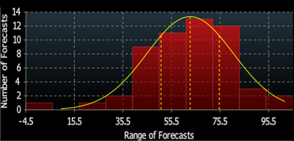
The consensus today is that the global economy, led by developed countries, is heading into recession in the next few quarters. The debate ranges between hard or soft landing. Bloomberg’s recession probability forecast stands at 65% today. To add to this bleak outlook, we have Fannie Mae and Visa, companies with real economy visibility, forecasting an 85% chance of recession.
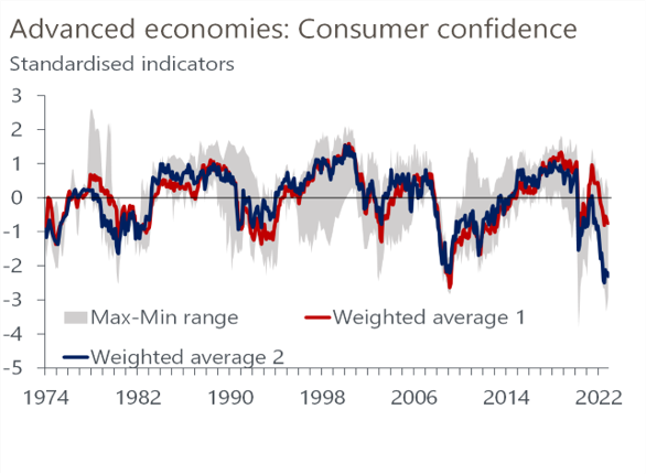
Some of this doom and gloom is based on the past relationship between surveys and hard data. Soft data points to the worst economic environment in half a century, only comparable to the Great Financial Crisis.
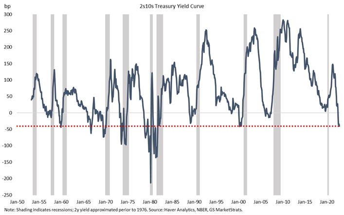
Financial markets are also forecasting an imminent recession when looking at the shape of the yield curve. The spread between 2-year and 10-year US Treasuries is the lowest since the high inflation period of the 1970s.
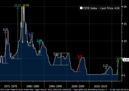
If we could point to only one data point to explain such dreary levels of survey responses and market pricing, it would be the speed and magnitude of the change in short-term nominal rates. The Federal Reserve hiked 425 basis points in nine months. This represents the fastest and largest rate-hiking cycle since the 1970s. The market and economists alike are saying that the current level of interest rates is incompatible with the economy’s structure. Markets believe that this level of rates will invariably cause the economy to contract, inflation to go back to 2% in the short- and long-term, and the Fed to start cutting rates in the second half of 2023.
The conclusion is valid if we accept the assumption that the trends of the 1985-2019 decades are still in effect, and that what we have seen over the past two years was just the effect of transitory impacts of Covid measures.
Having said that, markets are already broadly pricing these assumptions with a reasonably high confidence level. As investors, we must ask ourselves, ‘what if?’ What if there is a deeper reason for the past two years’ economic dynamics? What if we are not living through (only) transitory effects? Then, looking at nominal rates to predict a recession and a turning point for inflation would be misguided. And if so, the US treasury market would have to reprice materially in 2023, causing a structural shift in the global economy and financial markets.
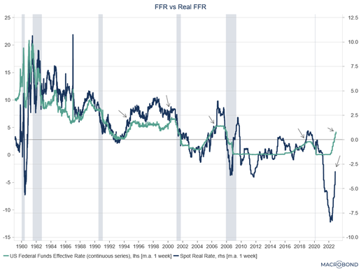
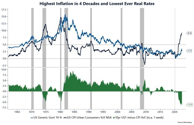
Inflation in the period from 1985 to 2019 averaged 2.6%. This is when we saw the third wave of globalization, increased working-age population, plentiful fossil fuel energy, and the unquestioned Pax Americana. With inflation at such low levels, one would be excused if all its conclusions were based on nominal rates assumptions. But inflation is only low sometimes. From 1950 to 1985, as well as from 2019 to today, inflation averaged 4.5%. When inflation is higher, nominal measures become less important and it is essential to look at real interest rates. Here, we use the Fed Funds Rate deflated by YoY CPI.
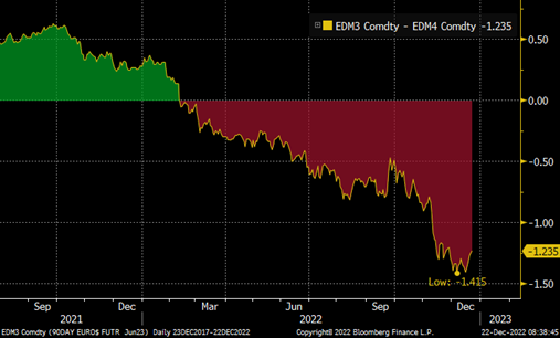
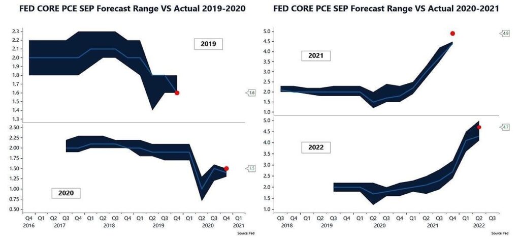
Real interest rates tell a very different story. We have seen a sharp increase in real rates since the beginning of 2022, but that move started from a historically low level. Today, real rates are still extremely negative, even after 425 basis points of hikes from the Fed in 2022. The conclusions we draw from looking at this measure are very different from those based on the nominal rate. We see a monetary stance that is not restrictive and, therefore, supportive of growth. With that, we also see the probability of recession at very low levels in the next few quarters, and little reason for the Fed to start cutting rates in the second half of 2023 (let alone the 125 basis points of cuts the market is pricing in between 2H23 and 2H24 – see graph below). This measure helps explain why the labor market is so strong, something that keeps confounding central bankers and analysts alike. It also helps explain why surveys are so pessimistic. In periods of inflation, people tend to have a very pessimistic view of the economy, even when real growth is positive.
We must then ask ourselves. What if real rates are more important for the economy than nominal rates? What if the structural trends of less globalization, a decrease in the working-age population, scarce fossil fuel energy, and a multipolar world materially increase R*? What if the recent weakness in inflation numbers is just a transitory effect as part of a long-term structural inflationary period? What if growth surprises to the upside in 2023, even with the Fed keeping rates above 5%? What if?
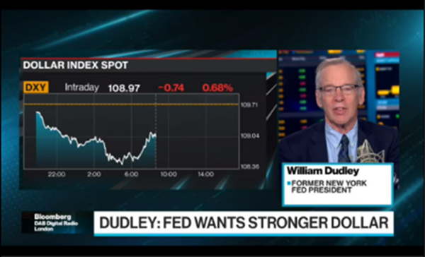
This past Friday, September 9th, Bill Dudley was on air early morning making the case that the Fed wants a strong dollar. We know very well why the Fed needs a strong dollar. We wrote on July 25th about the relationship between inflation expectations and the currency’s strength:
“The DXY Dollar index is more than 17 percent up YoY, while the US CPI is 9.1 percent. Being conservative, we can assume a short-run currency passthrough in the US at about 25 percent. This means that if the US Dollar was flat year-over-year, inflation should be a whopping +13%! This blind faith in central banks is what is keeping everything together.” – Macro Minute: We Learn From History That We Do Not Learn From History. July 25th, 2022.
However, how long the Fed can enjoy this position is less clear. Free-floating exchange rates, as opposed to the traditional view that expects a move to equilibrium at fair value, are inherently unstable. The reason for that is the reflexive nature of exchange rates. A change in exchange rates affects inflation, interest rates, economic activity, and other fundamental factors that then have an impact on exchange rates. This effect creates self-reinforcing and self-defeating processes that are very pronounced in currency markets.
In the case of the US dollar today, the fundamentals and nonspeculative transactions point in the direction of depreciation. It is only when looking at speculative transactions that we can find an explanation for the strength of the dollar in the past 12 months. In reality, the classification of speculative and nonspeculative is much more subtle, but for the purposes of this analysis, a simplified version of the model should suffice.
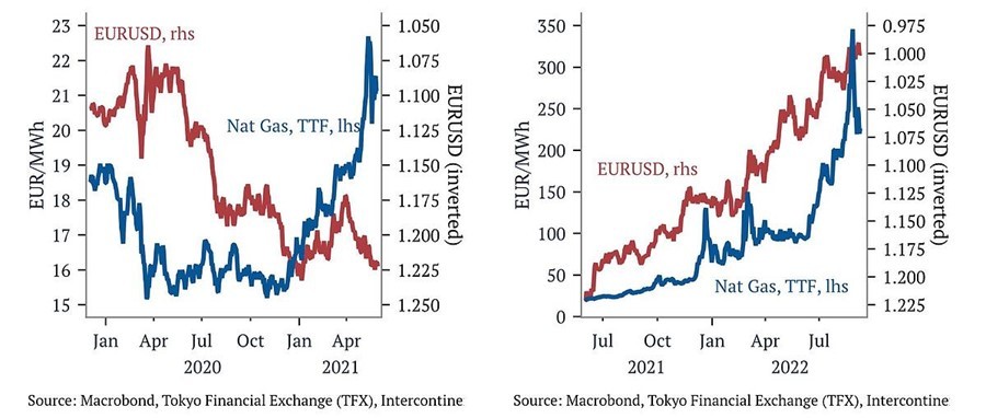
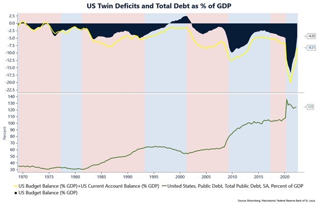
Non-speculative capital flows arise from the need (not the choice) to buy or sell dollars. On this account, all the fundamentals point towards the depreciation of the US dollar. The need to finance the US twin deficits is not new, but it has increased meaningfully recently. But one component in particular is seeing the largest changes- the need for USD in commercial transactions. Charles Gave, co-founder of Gavekal, wrote an excellent piece on “Network Effects and De-globalization.” In it, he proposes that reserve currencies benefit from the network effect, and that the turning point for the demand for US dollar transactions happened when the US insisted upon oversight of all US dollar transactions anywhere in the world. He argues that the catalyst for accelerating the contraction of this network was the US sanctioning Russian assets earlier this year. This decline has so far been masked by an increase in demand for USD coming from the energy crisis in Europe. We agree with that analysis and we can see the relationship between natural gas prices in Europe and the EURUSD (inverted axis) pre and post-mid-2021 below.
Speculative capital, on the other hand, is attracted by rising exchange rates and rising interest rates. Of the two, exchange rates are by far the most important. It does not take very large movements in exchange rates to render the total return negative. In other words, speculative capital is motivated by expectations of the exchange rate, a reflexive process. And when markets are dominated by speculative flows, they are purely reflexive. This is a very unstable situation. The self-reinforcing process tends to become vulnerable the longer it lasts, and it is bound to reverse itself, setting in motion a process in the opposite direction.
This is an obviously oversimplified model, but it brings useful conclusions. When the inflow of speculative positions cannot keep pace with the trade deficit, rising interest obligations, and lower demand for trade in US dollars, the trend will reverse. When that happens, the reversal may accelerate into freefall, as the volume of speculative positions is poised to move against the dollar not only on the current flow, but also on the accumulated stock of speculative capital. Lastly, when that happens, the exchange rate will have an impact on fundamentals (inflation and inflation expectations) which in turn will have an impact on exchange rate expectations in a self-reinforcing process. All of this will make the Fed’s job that much harder.
Given the unpredictable nature of speculative flows and self-reinforcing trends, we can’t say for certain when this will happen, but if pressed for an answer, I would say in the next 9 months. If the US dollar maintains or accelerates its trend during this period, the EUR would have to be trading below 0.86, the JPY above 170, and GBP below parity. And if it doesn’t, the reversal would be dramatic, if not catastrophic.
Last week, just before the end of the month, we got the Second Quarter Advance GDP Estimate from the US Bureau of Economic Affairs (BEA). The quarter-over-quarter annualized number for real GDP printed a disappointing -0.9%, compared to a median expectation of +0.4%, but still better than the 1Q number of -1.6%.
GDP releases are very important events for markets. Companies use them to help make investment decisions, hiring plans, and forecast sales growth. Investment managers use them to refine their trading strategies. The White House and Federal Reserve both use GDP as a barometer for the effect of their policy choices.
These numbers are especially important for turning points in the economy. For some (but not the National Bureau of Economic Relations – the US agency responsible for classifying recessions), two consecutive quarters of negative real GDP growth is defined as a recession. If we took the early GDP releases at face value, this would imply that we are in a recession today, dating back to the first quarter. For all the above reasons, it is worth digging into how the BEA derives this number and how reliable the early releases are.
One of the tasks of the BEA is to calculate US GDP, measured as the total price tag in dollars of all goods and services made in the country for a given period. It is the sum value of all cars, new homes, lawnmowers, electric transformers, golf clubs, soybeans, barbeque grills, medical fees, computers, haircuts, hot dogs, and anything else sold in the US or exported during the period. When calculating current (or nominal-dollar) GDP, the agency adds the value of all goods and services in current dollars. But this herculean task does not end there, because what matters for most people is the real growth in the economy. And so, after tallying up everything in current dollars, the agency has to then make adjustments to try and come up with an estimate of the value of what was actually produced in the economy (e.g., ex-inflation).
Imagine an economy that only produces two things, potato chips and mobile phones. Suppose that the economy is selling $1.1 million of goods this year, an improvement of 10% compared to the $1 million from last year. That $1.1 million number represents the nominal GDP for the economy this year. But that number does not tell us how much of that 10% increase is due to more goods being sold and how much derives from price increases.
If last year there were 50,000 bags of chips sold for $10 and 500 mobile phones for $1,000, and this year there were 55,000 bags of chips and 550 mobile phones sold for the same price as last year, the economy had real growth of 10% and zero percent inflation.
Alternatively, if this year the economy sold the same number of chips and mobile phones as last year but did so at a price of $11 and $1,100, respectively, the economy had zero real growth and 10% inflation.
However, things are not so simple, for the methodology is designed not only to remove price inflation but also to adjust for the quality of the goods being sold. Let’s assume that this year the economy sold 55,000 bags of chips for $10, and 550 phones for $1,000 (the same as the first example). But in this example, the bags of chips sold this year only contain 40 chips versus the 50 chips in each sold last year, and the mobile phones sold this year have better computational power and an extra camera versus last year’s. In this case, the agency would have to account for those changes by calculating a positive price increase for the potato chips and a negative one for the mobile phones, even though the number consumers saw on the price tag did not change. Now imagine that the BEA must do this not just for all the goods sold in the US economy, but also for every service provided, and to deliver an advance estimate one month after the end of a quarter.
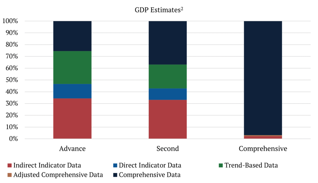
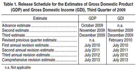
Which brings us to the question, how reliable are early GDP estimates? The answer is… it depends. Each revision incorporates more and better data and is believed to be a better estimate of the true value of GDP. For example, comprehensive data accounts for only 25.5% of advance estimates and 36.8% of second estimates, but it accounts for 96.7% of what we can call “final” estimates[1].
To assess the reliability of the GDP estimates we can look at revision patterns to understand if there is a bias in these revisions and how large they can be. To assess bias, we calculate Mean Revision (MR) where components tend to be offsetting and a large positive or negative number would indicate bias. To understand how large revisions can be, we calculate the Mean Absolute Revision (MAR) and the standard deviations, which are both complementary measures of the distribution for the revisions around their mean. We calculate these revision metrics for the Advance release that comes out one month after the end of a quarter, comparing with both, the Second releases (two months after the end of a quarter) and what we here call the “final” estimates (also called, comprehensive revisions, which are released approximately five years after the advance release).
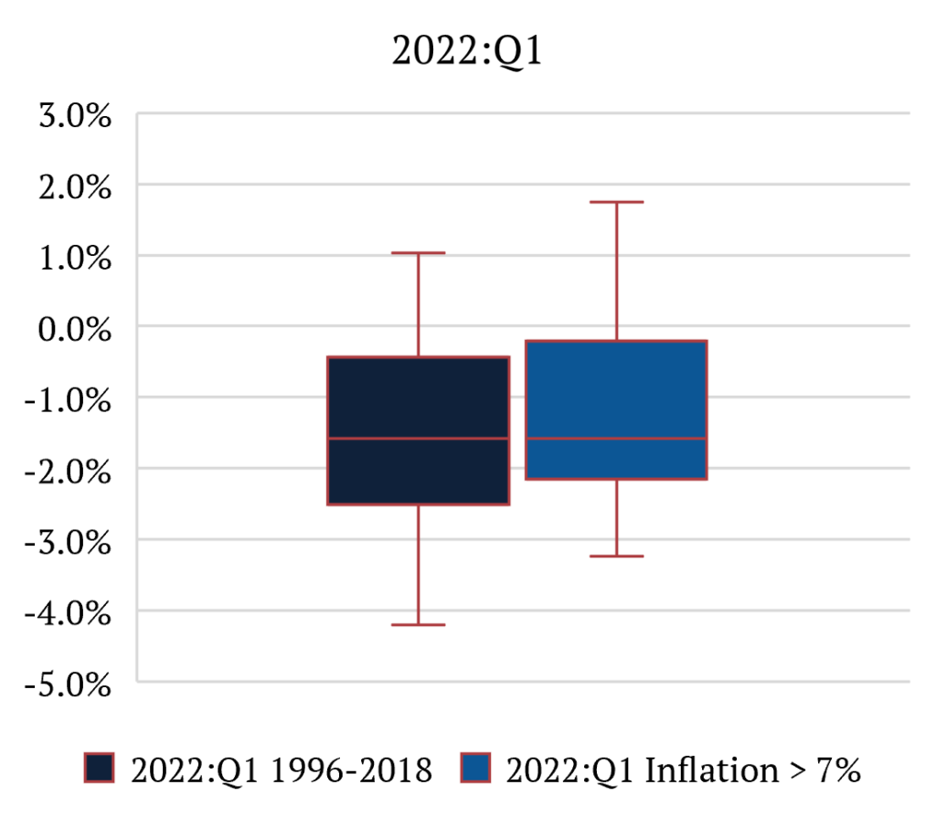
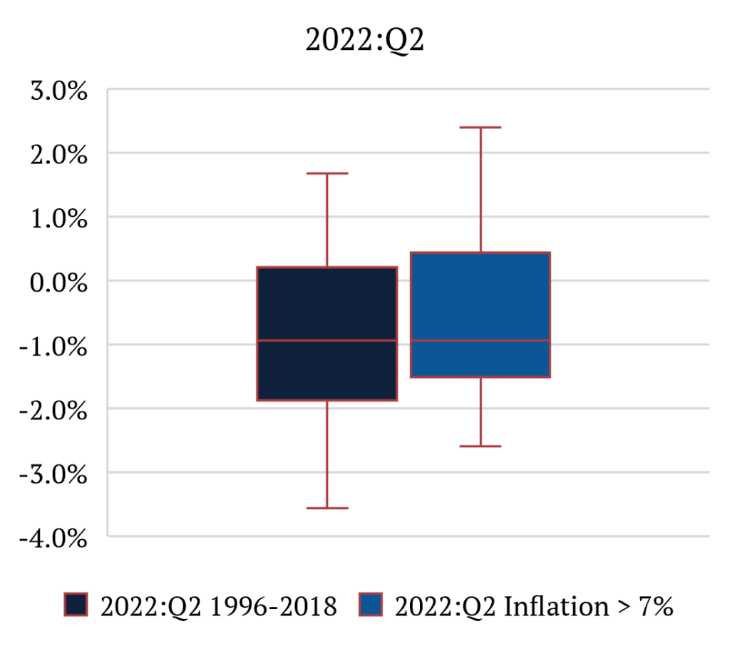
What we find is that inflation has a meaningful impact on reliability. More specifically, it creates a pronounced bias for advance releases in underestimating real GDP growth. This makes intuitive sense. The task of calculating real GDP becomes even more challenging during inflationary environments. Looking at the numbers, we find that in periods of low inflation [3,4], bias is virtually inexistent with MRs for Second and Final at +0.10% and -0.01%, respectively. While during periods when US CPI is above 7%, MRs are +0.40% and +0.80%, respectively. That means that, on average, in high-inflation environments, Advance GDP numbers are underestimated materially. It is also important to note that MARs and standard deviations are essentially unchanged from one environment to another. This means that the size of revisions is similar in both circumstances.
To clarify the point, let’s look at last week’s 2Q 2022 GDP Advance release of -0.9%. We can say that the second estimate will be between -1.5% and +0.4%, while the final estimate will be between -2.6% and 2.4%, with 90 percent confidence. This distinction between inflationary and non-inflationary environments is important because if we used the low-inflation scenario numbers, we would say that the second estimate would be between -1.9% and +0.2%, while the final estimate would be between -3.6% and +1.7%, with 90 percent confidence. [5]
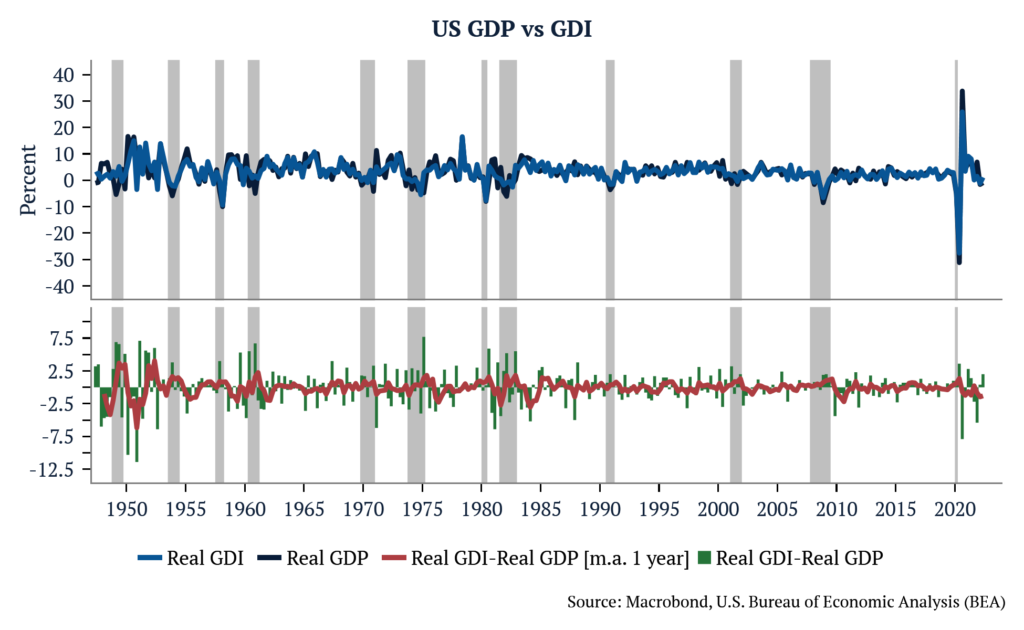
One way to increase the reliability of activity numbers is to look at the average of GDP and GDI. In theory, GDP and GDI should be equal, but in practice, GDP and GDI differ because they are constructed using different sources of information – both are imperfect in different ways. If both GDP and GDI are interpreted as the sums of unobserved, true economic activity and measurement errors, it is possible to infer that the weighted average series of the two is a more reliable measure of activity than either GDP or GDI alone, assuming some of the measurement errors are averaged out.
In short, calculating GDP is a mammoth undertaking, early estimates of real GDP tend to underestimate growth in inflationary environments, and you are better off taking a holistic view of the economy when data is as volatile as it is today.
P.S. We talked a lot about real GDP, but we should not neglect nominal GDP. Historically, S&P earnings growth tended to stay in line with nominal GDP. And that is how corporate sales, revenues, and profits are recorded. In the second quarter of 2022, nominal GDP in the US was approximately +7.9% QoQ annualized.
P.P.S. For a depiction of how and when GDP revisions and their vintages are made and maintained by the BEA, please see below.
[1] Comprehensive revisions are performed every five years and include major updates to classifications and definitions for the entire GDP time series – for more information, please see the endnote
[2] Holdren, Alyssa – Gross Domestic Product and Gross Domestic Income – Revisions and Source Data (June 2014)
[3] Fixler, Francisco, Kanal – The Revisions to Gross Domestic Product, Gross Domestic Income, and Their Major Components (June 2021)
[4] Using 1996-2018 period used in above paper, when US CPI inflation averaged 2.2%
[5] Revisions follow a normal distribution and therefore we can calculate the combined probability that the true value of real GDP growth in the 1Q and 2Q was below zero, i.e., two consecutive quarters of negative GDP growth. P (2Q < 0% | 1Q < 0%) = 36%.
Despite all the efforts of the most brilliant economists and analysts in the world to build models mimicking the methods of physics that follow their own self-contained logic, rules, and patterns to predict outcomes, when faced with failure, they dismiss it by claiming that “random shocks” had somehow disturbed equations and did not need to be explained since they are “nonrecurring aberrations.” War, pandemics, and politics are not abnormal historical events, only in economics.
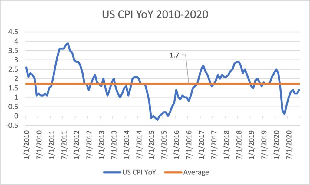
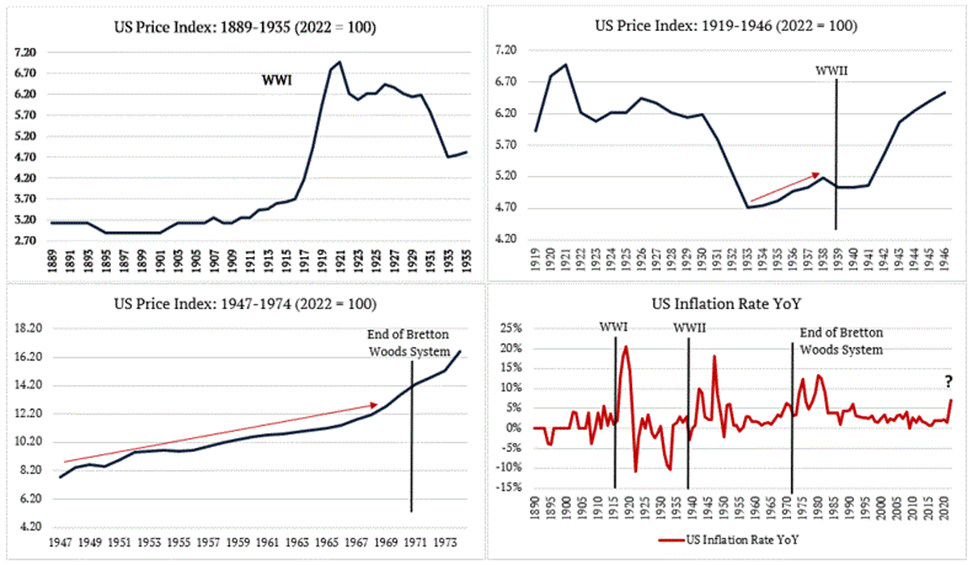
However, many questions in economics can be approached more simply through history. In the most recent record, from 2010 to 2020, US CPI YoY averaged only 1.7%, below the Fed’s target (how much did that play a role in the recent late response from the Central Bank is anyone’s guess). However, in the history of the US, there are only a handful of times that the inflation picture could be described as stable.
Looking back at American history, we find six inflationary spiral events. The first occurred in the late 1700s just after the Revolutionary War; the second in 1813 after the War of 1812; the third in the 1860s during the Civil War; the fourth in the late 1910s after World War I; the fifth around and after World War II in the mid-1940s; and, the most current one in the 1970s associated with the Vietnam War. These periods were always followed by long periods of deflation. Evidence would point to politics, not economics, to explain inflationary spirals, and war looks like the common denominator. War in itself has many different impacts on inflation (as we discussed in this Macro Minute: The Reflexivity of Inflation and Conflict). Still, it is really the increase in money spent by the government, above what it collects in taxes, that makes inflation and negative real rates an attractive solution to the debt problem.
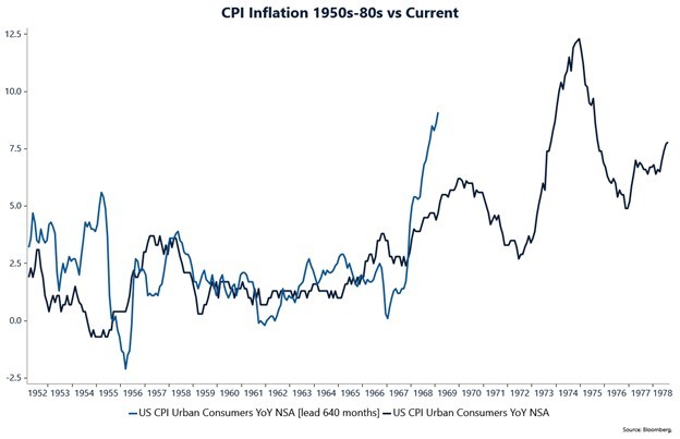
Looking back to the latest inflationary cycles of the 1970s, we find a few similarities and one significant difference. [1]
Similar to the present day, in 1975, the government balance sheet resembled conditions only tolerated during periods of war. And in the preceding years, just like recently, conservative governments that were supposed to be fiscally conservative were actually accelerating the deficit. In today’s world, for example, if interest rates rise above inflation, the Treasury’s interest expense goes up as debt rolls over, and the Fed reduces remittances to the Treasury. The Congressional Budget Office calculates that a 1% increase in real rates increases the annual deficit by $250 billion, about 1% of GDP, planting the seeds for an explosive debt dynamic.
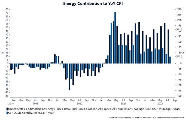
In the 1970s, oil price inflation was a big problem, increasing to around 6 percent per month. More recently, on average, oil has been growing at 4.2 percent per month since January 2021. That includes the price corrections we saw in the last couple of months. The contribution to the CPI is still high at 47% YoY at current gasoline prices.
In the 1970s, real interest rates reached -4 percent. Today, we are living through the most extended period of negative real rates, currently sitting at -6 percent. That is before factoring in what can happen with nominal rates in a recessionary scare. We calculate real rates by subtracting the US Treasury 10-year yield by the current CPI YoY number. We believe this is a better indicator of real rates on Main Street than the real rates derived from the TIPS markets on Wall Street. This is the rate that alters the lives and actions of people who are not traders or advisors and who do not follow the FOMC decisions or read the Wall Street Journal. Different from the previous cycle, when the Fed was focused on impacting asset prices, to have an impact on goods and services prices, the central bank needs to focus on the decisions in the real economy and not in financial markets.
“At 15 percent inflation, an investor lending $1 million at 10 percent ‘loses’ $50,000 a year. You cannot count on the lender being a complete idiot, sooner or later, he will stop lending at low-interest rates and invest the money himself in commodities or real estate.” – Senator William Proxmire. October 1979
Another interesting observation from looking at real interest rates is that every recession is proceeded by positive real rates. More importantly, real rates tend to turn negative to help the economy once a downturn starts. This brings us to the recessionary debate. Like today, in 1979, most economists, including the Fed, were forecasting a recession. They had been wrong for many months, and in September, data showed the economy was not tipping over; it was accelerating again. This was true even with a deceleration in housing and autos and the fear of recession. “A Gallup survey found that 62 percent of the public expected a recession sometime in 1979.”
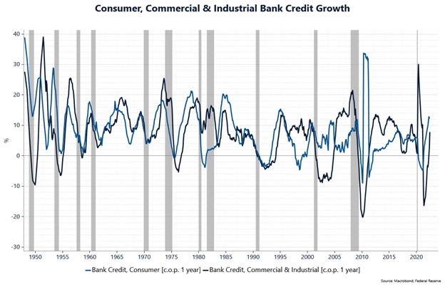
In an inflationary economy, people behave differently. Inflation doesn’t slow people down. With inflation at 16 percent, borrowing at lower rates seemed like a good deal. Bank credit was expanding at an annual rate of 20 percent. Most consumers did not care about what the higher interest rates were, as long as the monthly payments could fit their incomes. This is not a foreign concept for Latin Americans.
“Lenders were still surprised at how many families were willing to take on home mortgages at 13 percent or even higher. ‘ Perhaps it is not so hard to understand,’ Volcker said, ‘when you realize that the prices of houses have been going up at 15 percent or more.’” – 1979
Today, bank credit is growing at +12% for consumers and +8% for Commercial and Industrial clients. We’ve been following bank’s earnings calls very closely and we find that all the major banks see strong balance sheets, very low forward-looking default rates, and expect credit to grow in the mid-teens for the next few quarters. This past week, American Express reported that overall cardholder spending rose 30% from a year earlier.
Even when the Fed was finally able to create the presumed remedy, a prolonged recession that endured for 15 months with unemployment rising to 9.1 percent and industrial production shrinking to roughly 15 percent, as soon as the economy recovered, inflation came roaring back, rising even higher than before even with employment never getting close to its natural rate. With the supply of commodities constrained, even a short-term decrease in demand does not fix the inflation problem; it only postpones it to the following part of the cycle when policies revert to accommodative.
Lastly, the Fed genuinely did not know how much interest rates would have to rise to break inflation. If record levels of rates were not fixing the problem, how high would rates need to go to do it? Nor did it have the political capital to do what was necessary. Volcker acknowledges, ‘We could have just tightened, but I probably would have had trouble getting policy as much tighter as it needed to be. I could have lived with a more orthodox tightening, but I saw some value in just changing the parameters of the way we did things. (…) it would serve as a veil that cloaked the tough decisions.’”
“There is a wide concern about the Fed’s resolve in adhering to this policy in the face of an election year and the increasing likelihood of a recession. If strong words and actions are not followed by results, then holders of dollar-denominated financial assets in the US and abroad will conclude that the recent changes are no more significant than the statements and policy changes of prior years which did not reduce inflation. When rhetoric sufficed several years ago, tangible proof is now required of the Fed’s intentions.” – Federal Advisory Council 1979
The similarities are striking.
The main difference between the 1970s and today lies in the credibility that central banks around the world collected during a period of global deflationary forces that made them look like they could bend prices to their will and achieve their dual objective effortlessly, giving rise to the mantra “Don’t fight the Fed!” On July 14th, 2022, Governor Waller said, “The response of financial markets to the FOMC’s policy actions and communications indicate to me that the Committee retains the credibility and the public confidence that is needed to make monetary policy effective. (….) lenders and borrowers are still doing business at these rates, which indicates that they believe the FOMC’s policy intentions are credible, as broadly reflected in the interest rate paths in the Summary of Economic Projections (SEP).” Today, markets price the Fed’s projections to perfection.
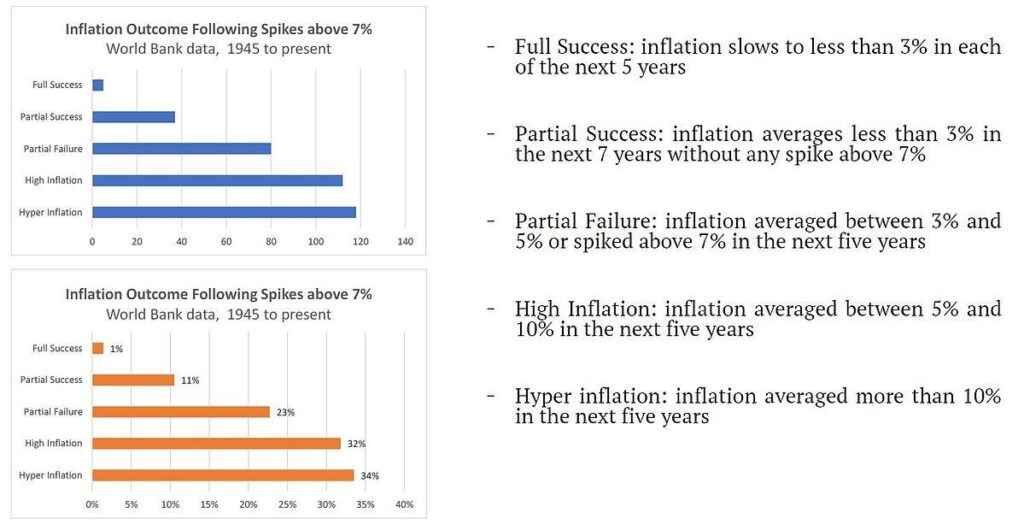
What does history tell us about that? StoneX’sVincent Deluard shows us that using post-war data from the World Bank of more than 350 events when inflation spiked above 7%, only 1.4% of the time, inflation slows to less than 3% in each of the next five years. Markets are pricing 1 in 70 odds as if it were 100 percent certain.
“Acting hastily is essential to [a trader’s] profitability. If today’s quickest-to-the-keyboard move makes little sense according to some notion of ‘fundamentals,’ who cares? Overshooting is a feature, not a bug.” – Alan S. Blinder, July 2022.
“Traders must and do therefore respond literally instantly to all news to which they think other traders might respond. Whether the news is considered economically significant or even true is immaterial.” – Albert Wojnilower, Chief Economist at First Boston 1964-1986
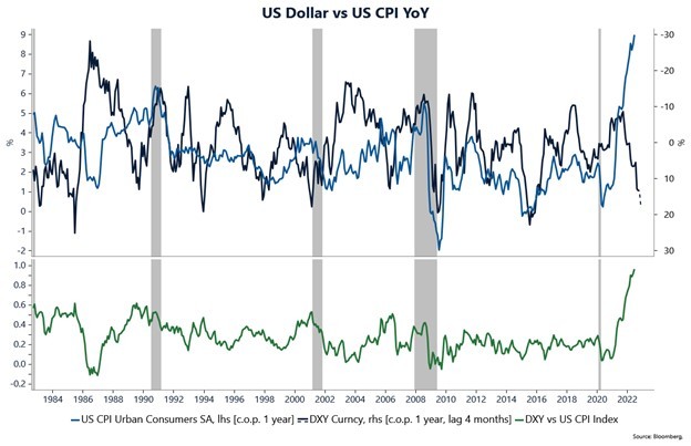
This confidence also has an impact on the USD. With the expectation that inflation will converge to 2% in the next 18 months, interest rate differentials make the currency attractive. That, in turn, keeps inflation in the US in check. The DXY Dollar index is more than 17 percent up YoY, while the US CPI is 9.1 percent. Being conservative, we can assume a short-run currency passthrough in the US at about 25 percent.[2] This means that if the US Dollar was flat year-over-year, inflation should be a whopping +13%! This blind faith in central banks is what is keeping everything together. But history also tells us that after a long deflationary cycle and the build-up in credibility, what comes next is the drawing down of goodwill until there is nothing left.
“We’ve lost that euphoria that we had fifteen years ago, that we knew all the answers to managing the economy.” – Volcker 1989
[1] A good friend of the firm and fellow investor, knowing of our quest to understand history, pointed out to us that the team at MacroStrategy research was studying a book written in 1989 by William Greider called “The Secrets of the Temple” about the Fed’s fight against inflation under Volcker to help them with a similar pursuit. This book has been invaluable in our understanding of the period, and all quotes in this letter are from the book. https://www.amazon.com/Secrets-Temple-Federal-Reserve-Country/dp/0671675567/
[2] Campa, Jose Manuel, and Linda S. Goldberg. “Exchange rate pass-through into import prices.” Review of Economics and Statistics 87.4 (2005): 679-690. (https://www.nber.org/system/files/working_papers/w8934/w8934.pdf)
Exchange Rate Pass-Through and Monetary Policy, Governor Frederic S. Mishkin, at the Norges Bank Conference on Monetary Policy, Oslo, Norway. March 07, 2008 (https://www.federalreserve.gov/newsevents/speech/mishkin20080307a.htm)
Takhtamanova, Yelena F. “Understanding changes in exchange rate pass-through.” Journal of Macroeconomics 32.4 (2010): 1118-1130. (https://www.frbsf.org/economic-research/wp-content/uploads/sites/4/wp08-13bk.pdf)
We believe that 2021 marked the beginning of a secular bull market in commodities and commodity-related equities, with the usual peaks and troughs along the way. A decade of underinvestment by producers and refiners of natural resources coupled with burgeoning excess demand for those resources driven by a myriad of global initiatives including electrification, food security, and energy independence has shifted the long-term supply-demand outlook into deficit for many commodities.
Going back to the 1970s, a period where many investors are looking for clues given the recent run-up in inflation globally, commodity prices and related equities enjoyed a bull market that only ended in 1980 with the collapse of a commodity bubble. In the early 1980s, oil prices began to drop, and at the same time the Federal Reserve was credibly moving to “break the back of inflation”. Since then, we lived through a constant cycle of disinflationary forces that ended in the mid-2010s.
Almost all crises since the 1980s were balance sheet crises, and therefore deflationary. The Japan bust, the Asian crisis, the sub-prime crash, and the Euro crisis were all balance sheet and banking crises. Those crises were deeply deflationary in an already deflationary environment. As balance sheets were negatively impacted, borrowers constrained consumption and investment to pay down debt, while at the same time banks constrained lending, which in turn negatively impacted the price of assets used to collateralize said debt, restricting banks’ ability to lend in a never-ending vicious cycle… until governments stepped in.
Global demographics served as a tailwind for labor and led to an increase in savings that got recycled into US Treasuries – colloquially known as the global savings glut. With the fall of the Berlin Wall in 1990 and China being admitted to the WTO in 2001, globalization went into overdrive as companies could tap into a global labor force, resulting in even more disinflation.
Equities and commodities have swapped market leadership in cycles averaging 18 years in length for over a century. Over time these cycles have become shorter with technological advancements, but they are still fairly consistent, predictable, and long. Commodity price bubbles tend to bust after military or economic conflicts due to the well-known “peace dividend” which drives lower commodity and input costs, better profit margins, higher equity multiples, and more leverage brought on by lower rates and a low-inflation environment. Conversely, when equity bubbles deflate, inflation resurges. Large amounts of debt that were accumulated during the expansionary phase must be reduced using a combination of inflation and defaults. When that happens, easy monetary policy follows, and military or economic conflict once again occurs, perpetuating the long-term cycle.
In the subsequent sections of this report, we examine in detail three probabilistic scenarios for what the medium- to long-term outlook in markets may be, but a summary of the analysis is as follows.
(1) Sustained growth and higher prices via re-leveraging of consumers, a renewed corporate investment cycle, and the build-up of inventories in a more inelastic supply environment. This view is anchored in the belief that the world is transitioning from slack to generally tight commodities supply. (P = 55%)
(2) Rising conflict, disruptions, and nonlinear upside price movements leading to a prolonged period of stagflation. Major wars (or other exogenous shocks like pandemics) produce high inflation, and even minor wars can interrupt trade. Conflict and inflation are intrinsically linked, especially coming out of a period of extreme money supply growth. (P = 35%)
(3) Continued price disinflation or deflation, western-dominated status quo, resumption of the technology capital expenditure boom, and prolonged strength for US equity index returns. In this scenario, the belief is that the Fed will not be as aggressive in hiking rates this cycle given the unsustainable divergence between rising debt as a percentage of US GDP and the falling nominal GDP growth derived from that debt. (P = 10%)
The above scenario analysis and applied probabilities shape our forward-looking market views and positioning. Throughout this report, we provide the economic data and analysis in support of these ideas, and a summation of the key points can be found below:
We believe that for at least the next few years, we are entering a new environment for inflation with consistently higher price levels. Some indicators to watch for are surging real estate prices, high money supply growth, large fiscal deficits, strong commodity prices, increasing geopolitical instability, and stretched valuations for the US dollar.
In that period, we also expect strong nominal GDP growth, while the outlook for real GDP growth is more uncertain given the rising risk of conflict or a central bank miscalculation.
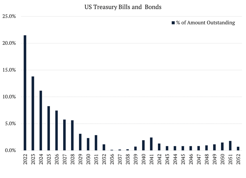
Rising inflation will lead to Fed rate hikes, but the governors may have little choice but to return to an accommodative stance due to the “hangover” of past financial excesses and, potentially, war. Government roll-over rate risk is very large, with approximately two-thirds of United States federal debt maturing in the next four years.
We expect strong global commodity demand and commodity prices to be a central theme as well. Poor profits have discouraged investment by commodity producers since the mid-2000s, and the growth of sustainability concerns has exasperated the underinvestment.
With supply already in short store, producers have moved from the last decade of short duration investment – restock, destock, capex binge, balance sheet distress, capital raise, boom, and bust – to longer duration, disciplined capex cycles.
As a result of these dynamics, we expect commodities to outpace the S&P 500 over the next few years. Commodities become a defensive asset in commodity-driven recessions.
We see single-digit compound returns for the S&P over the period. The first part of the period will see negative returns and the later part low positive returns, as the focus shifts from multiple compression and falling earnings to cheaper valuations. Free cash flow generation will be key in both phases.
Inflation could be made significantly worse if increasing geopolitical instability leads to wars.
Given this outlook, we have built positions across the commodity complex, the core ones being in industrial metals – namely copper, aluminium, and cobalt – emission allowances, and grains. Alongside those positions, we have further built upon the theme through equity allocations to global energy refiners investing in renewable fuels (e.g., sustainable aviation fuel, renewable diesel), miners and refiners of industrial metals who lead in low carbon intensity production, and industrial companies exposed to the renewable revolution with large market share and pricing power. We expect the supply-demand fundamentals facing commodity markets to persist for many years, pressuring prices and having a negative impact on prevailing market sentiment, with a particular emphasis on long-duration assets. We will be hedging a portion of our equities exposure by betting against indices we find to be richly valued given our probability-weighted scenarios. We expect interest rates, especially in the developed world, to make higher highs and higher lows over the next few years, a quasi-mirror image of the lower highs and lower lows of the deflationary past few decades. Lastly, we believe that the currencies of commodity-exporting nations will benefit greatly from this scenario.
To arrive at these views, we have done extensive research that involves proprietary information and third-party data. If you are interested in a full copy of the report, please contact ir@norburypartners.com.
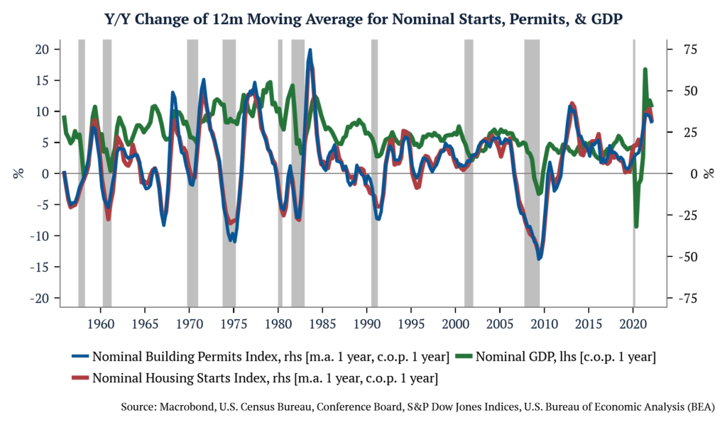
With so much talk about a recession lately, it is hard not to look for clues in housing numbers. This past week, we had numbers for US housing starts and building permits. While homes only directly account for roughly 5% of GDP, related goods and services can account for nearly 20%. Aside from 2001, the US has never gone through a recession when housing is doing well. Conversely, the US has never emerged from a recession without the help of housing (2009 being the exception with a rebound while housing was stagnant). Fort these reasons, it comes as no surprise that so much attention is given to the release of housing data.
Housing starts record how much new residential construction occurred in the preceding month, while building permits track the issuance of construction permits. The number for both releases is reported in number of units, with the latest number for housing starts and building permits disappointing the Bloomberg median survey at 1.549 million and 1.695 million, respectively. But how disappointing are these numbers, if at all?
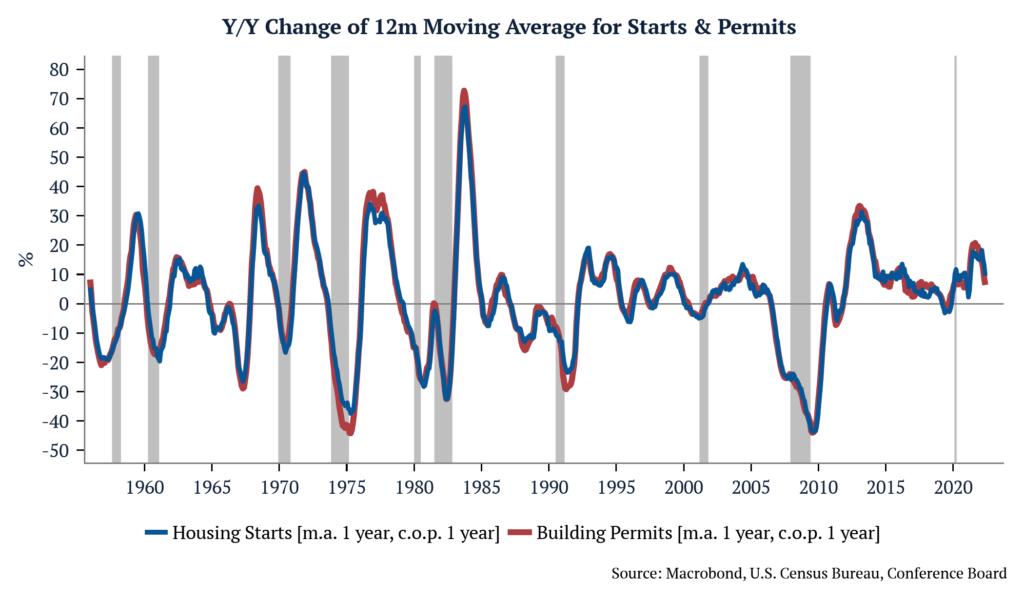
First, let’s look at housing starts. The month-over-month number came in at -14.4%, and comparing the latest release with the same time last year, the number of starts contracted by -3.5%; however, these numbers are very volatile and prone to significant revisions. When looking at the rate of change of the 12-month moving average in May versus the previous month, we encounter only a -0.28% contraction, and when comparing the average with the same period last year, we find a growth of +9.5%. Building permits decreased by -7% MoM and increased +0.2% compared to last year. Using the same 12-month moving average to smooth volatility, the rates of change from the previous month and last year are +0.2% and +6.4%, respectively. We can see some deceleration, but we are still at very healthy levels compared to the past.
One thing to keep in mind is that looking at housing starts and building permit numbers only gives us an idea of the real component of the economy. But for prices and company earnings, it is Nominal GDP that matters. Therefore, we have constructed a nominal index for housing starts and building permits using the S&P CoreLogic Case-Shiller U.S. National Home Price NSA Index. When looking at that number, we see some deceleration, but in aggregate both starts and permits are still running at very high growth rates.
We cannot draw firm conclusions from a single piece of evidence, but what a closer look at housing starts and building permits shows is that the probability of recession may not be as high as one perceives from reading headlines.
On a macroeconomic level, inequality can affect economic growth, productivity, and political stability, which in turn has direct implications for corporate profitability.
As with most social science endeavors, there is a healthy debate about the precise impact of inequality on growth. For starters, does it hinder or accelerate economic growth? Economic theory shows that with higher income and wealth come higher savings rates and, therefore, a higher level of investment and gross domestic product. In this case, if marginal productivity is higher for capital than for labor, one can see that more inequality would create higher economic growth. Also, in economies with underdeveloped credit markets, significant investments can only be made if wealth is accumulated. In the presence of imperfect capital markets and indivisibility of investments, an economy with higher levels of inequality may be able to introduce new industries, technologies, and markets and ultimately grow faster than the same economy with lower levels of inequality. Finally, there is an argument that reducing inequality reduces incentives to accumulate wealth through labor, entrepreneurship, and innovation, having, therefore, a negative impact on long-term growth.
However, a healthy debate should not be confused with a balanced debate. The bulk of the literature supports the theory that inequality hurts economic growth. Studies that found a positive relationship between inequality and growth were focused on the short term, and studies that found a negative relationship were focused on the long term. In other words, inequality can produce a small contribution to growth in the short term but will substantially adversely affect growth in the long term. Empirical results have increasingly supported the arguments for impaired economic growth and a negative impact on productivity in the face of rising inequality.
Poor people without access to credit markets often defer health care treatments, cannot procure housing or transportation and lack the means to further their education. This results in missed opportunities and diminished productivity and growth potential. The same applies to poor parents with multiple children compared to wealthy parents with few children. The inability of low-income families to invest in their children’s education, and the inability of poor workers to invest in developing job skills because of either financial constraints or time constraints while working multiple jobs, can result in a reduction in overall skills and knowledge of the potential employee pool. That can have a drag on growth, productivity, and business performance. Finally, there is the problem of the indivisibility of consumption. In the absence of developed credit markets, expensive items can only be acquired by accumulating wealth. If the economy became more equitable, part of the population initially excluded from the acquisition of these goods would enter the market, encouraging the creation of new domestic industries.
Societies with higher levels of inequality also tend to have higher levels of crime, keeping a larger share of the labor force from productive activities and decreasing potential growth. Also, with the increase in social instability, trust and social cohesion can erode, leading to conflict, political crises, and the resulting retraction of investments. One of the potential consequences is the rise of nationalism and the splintering of support for globalization. This scenario has played out in economies around the world over generations. Ray Dalio, the founder of Bridgewater Associates, the world’s largest hedge fund, has warned of the corrosive effects of inequality on faith in capitalism and, therefore, the stability of the institutions and markets in which business operates.*
*This excerpt appeared in the article “Business Risks Stemming from Socio-Economic Inequality” by Todd Cort, Stephen Park, and Decio Nascimento at the Columbia Law School Blue Sky Blog published on April 15, 2022. The article is based on the paper “Disclosure of Corporate Risk from Socio-Economic Inequality” by the same authors published on March 18, 2022. You can find the article here, and the paper here.
In The Changing World Order, Dalio makes the point that history shows us that empires follow a predictable cycle of rising and decline that he termed Big Cycle. The cycle starts at “The Rise” phase when there is strong leadership, education, character, civility, and work ethic development. Innovation is also enhanced by being open to the best thinking in the world. This combination increases productivity, competitiveness, and income. At “The Top”, the country moves from “growing the pie” to “splitting the pie”. While the country enjoys higher standards of living, people get used to doing well and enjoy more leisure time in detriment of hard work. Financial gains come unevenly, and the elites influence the political system to their advantage creating wealth, value, and political gaps. Borrowing grows to make up for the loss in productivity, weakening its financial health. “The Decline” happens when debt is large and there is an economic downturn leaving the country two choices: default or printing new money. Typically, countries opt for new money. The faster the printing occurs, the faster the deflationary gaps close and worrying about inflation begins.
It is clear that major wars are greatly inflationary, and even minor conflicts can interrupt trade, causing disruptions and increasing prices. But what we’re finding out is, inflation actually precedes periods of war or economic warfare.
It should come as no surprise then that the global increase in general prices along with a strong price increase of commodities is leading the world to a new era of conflict. Ukraine and Russia are not just material in the global trade of wheat but now also make up close to 20% of the world corn trade. A prolonged conflict can lead to issues this spring when planting starts causing significant productions shortfalls when harvest comes later this year, causing prices to go higher, increasing the risk of an escalation and conflict. This self-reinforcing process we see between inflation and conflict has a name, reflexivity. [1]
[1]The theory of reflexivity in financial markets was proposed by George Soros. Considered by most as one of the best macro investors in history, delivering an average annualized net return of 33% from 1970 to 2020. His work around the theory of reflexivity first appeared in his 1987 book “The Alchemy of Finance”. Soros’ theory of reflexivity is based around human fallibility—human beings can be wrong in their beliefs about the world and therefore act based on misguided knowledge. Heavily influenced by Karl Popper’s account of the scientific method (Popper was Soros’ tutor at the LSE), Soros argues that when the subject of study involves thinking participants, the scientific method must be changed to account for that fact. When thinking participants try to understand a situation, the independent variable is the situation. And when participants try to make an impact on the situation, the independent variable is participants’ views. Reflexivity occurs when the participant’s view of the world influences the events in the world, and these same events will influence the participants’ view of the world. When reflexivity is in play, it can cause boom/bust processes—self-reinforcement that eventually becomes self-defeating. For a detailed description of reflexivity and the construction of social reality, read “When Functions Collide” at https://www.norburypartners.com/nascimento-decio-when-functions-collide/
On February 1st, at Credit Suisse’s 2022 Latin America Investment Conference, Enio Shinohara moderated a conversation with Rogerio Xavier from SPX and Luis Stuhlberger from Fundo Verde. In it, Luis made a very interesting remark on the US interest rates curve, which loosely translates from Portuguese to “so far in the United States, the increase in interest rates being priced by the market has simply anticipated a series of hikes, but has not changed the terminal interest rate. In other words, the first probability that appeared during the pandemic was for the first hike to happen in 2023 or 2024. In the past year, these expectations were repeatedly pulled forward. It started with one hike in 2022, and now we are talking about 5 to 6 hikes of 25 bps in 2022. But the terminal interest rate has not changed; the terminal interest rate is around 1.80%. In my opinion, and I agree with Rogerio, this will not be enough.” (I highly recommend watching the entire conversation, especially if you have any interest in Brazil: English Link, Portuguese Link).
Central banks around the world have one big problem today – inflation. This issue is even more apparent in developed markets that are mostly seen as behind the curve. From traditional macroeconomic models, we know that central banks can restrict the supply of money to ease pricing pressures; however, there are a few ways that this can be achieved. The two most common approaches are hiking short-term interest rates and pressuring long-term rates higher, both with meaningful, but different, redistribution effects. Historically, hiking short-term rates has been the method of choice at the Fed. That was also communicated at the last FOMC meeting and markets are pricing for it. Nevertheless, the situation is fluid and central banks, especially the Fed, may conclude that influencing long-term rates might be a better tool for the current environment and their updated mandate that now includes improving inequality.
The traditional way of relying on short-term interest rate hikes to lower inflation has the effect of controlling prices of goods by curbing demand through a flat or inverted interest rates curve, thereby causing a recession that generates the necessary slack to keep prices from rising. This method acts through raising unemployment and having little effect on asset prices. As Luis mentioned, hikes have only been anticipated with minimal impact on long-term rates, which in turn had little effect on mortgage rates and equities. In other words, this method exacerbates inequality. This is what the market is pricing today, with forwards implying an inverted curve in the US and Europe one year from now.
We believe that once this becomes apparent, the Fed will move into a more aggressive posture regarding balance-sheet reduction and steepening of the yield curve. Central banks have tools to control term premia, and by doing so can influence mortgage rates and asset prices. By increasing mortgage rates, they can keep home prices in check and consequently OER, with the added bonus of improving affordability. By decreasing asset prices, they might be able to bring early retirees back into the labor force (due to the decreasing values of their nest eggs), slowing, but not reversing wage growth, and consequently keeping services inflation tamed. Since we are not going through a balance-sheet crisis, central banks can engineer a soft landing without killing growth by pressuring long-term rates higher. This method would potentially have a positive impact on inequality. We hold a strong view that the probability of this scenario is higher than what the market is pricing.
This week, we will once again touch briefly on labor force participation and attempt to make sense of the US Employment Situation Report from Friday.
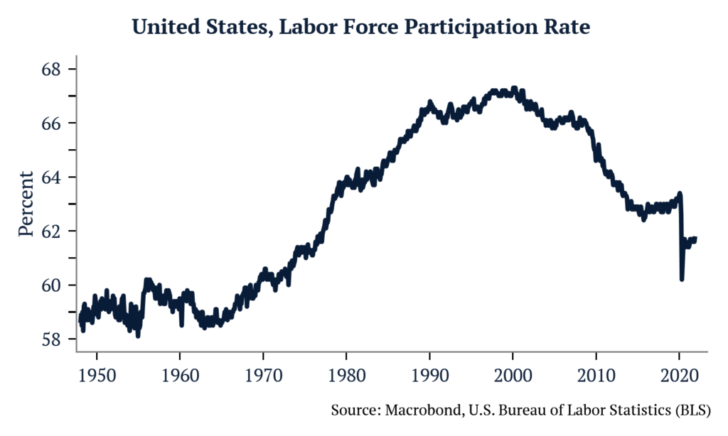
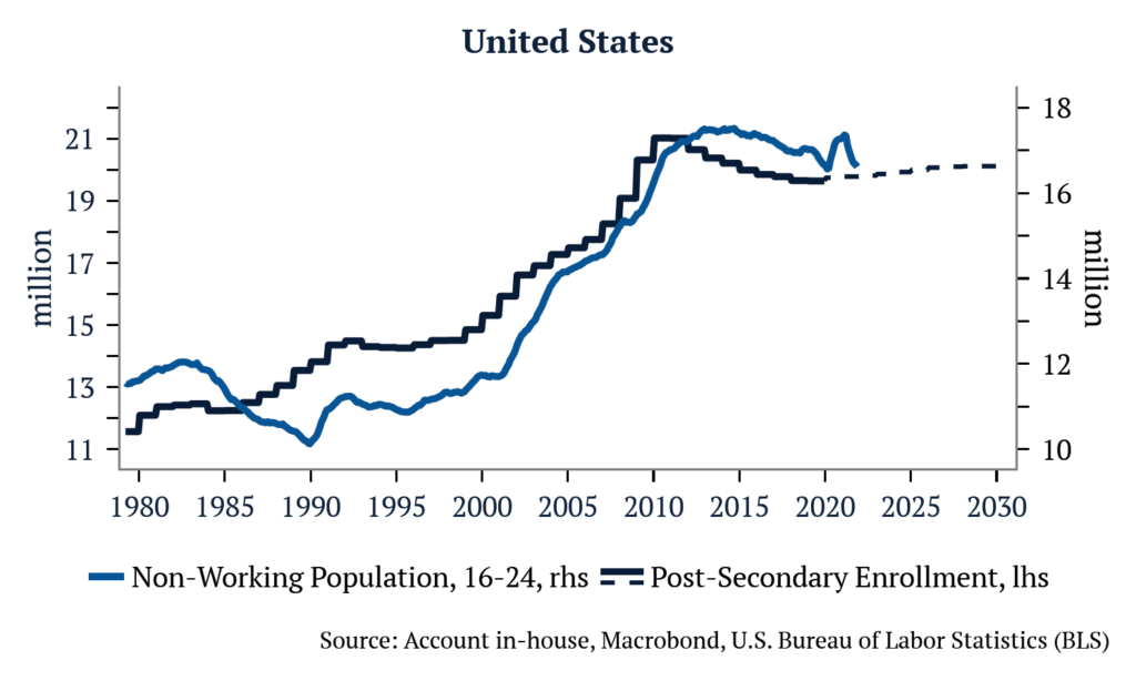
US labor force participation has been the subject of much discussion lately. Beginning in the 1960s when more women entered the workforce, it has steadily risen, moving from 59.1% to 66.9% by the year 2000. Since then, it has drifted lower and settled near 63% pre-Covid. A drop of almost 4% on the labor participation rate is equivalent to around 10 million jobs. At first glance this seems negative, but we find that most of this was due to strong levels of enrollment in post-secondary education among those aged 16 to 24. This trend began in the late 1980s, and accelerated into the 2000s, hence a deluge of social science majors and a dearth of truck drivers.
Turning to today, let’s analyze some of the most common arguments for explaining the slow recovery of the labor force participation rate.
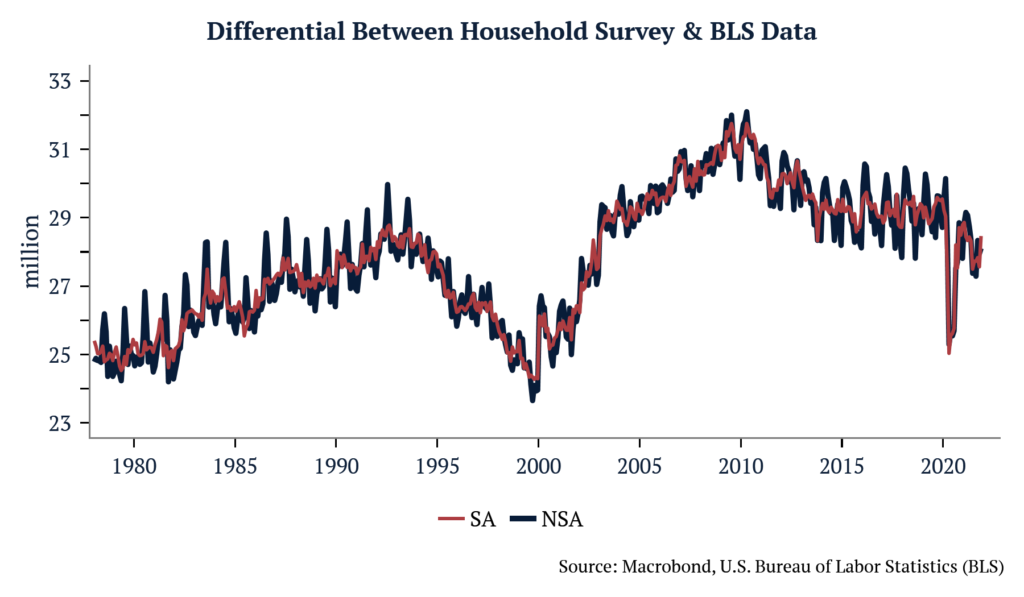
(1) Self-employment is keeping labor participation low – One way to try to test for that, is to track the difference between the household and the establishment employment data. The household employment figure captures the self-employed, farm workers and domestic help, something the BLS payrolls survey doesn’t do. Here what we find is that household employment suffered more than payrolls during 2020, and still hasn’t recovered to pre-covid levels.
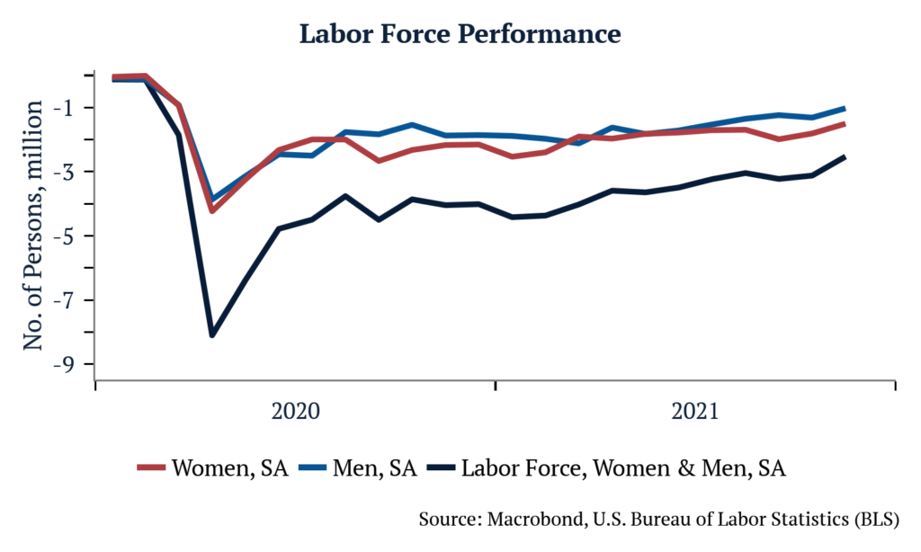
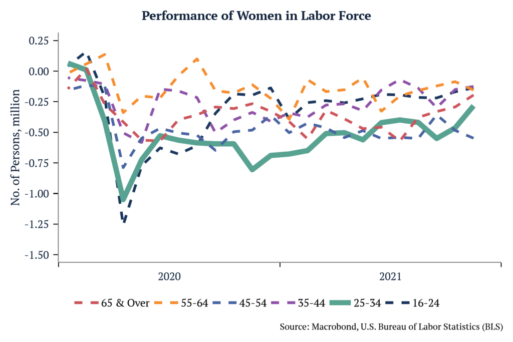
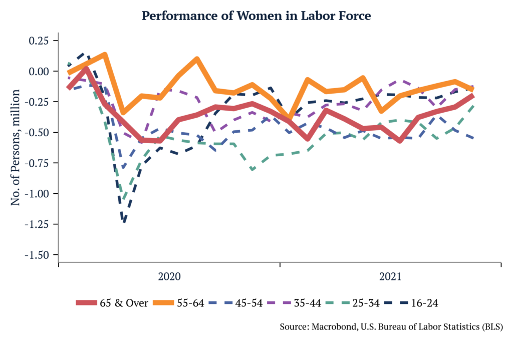
2) Women have been kept out of the labor force because of childcare– There is some indication this may be true. We saw nearly the same number of exits from the labor force for men and women in 2020 (3.9mm & 4.2mm in April ’20, respectively). Those aged 25-34 were the second most affected at the time, accounting for more than 1mm women exiting the labor force. By September 2021, there were still 550k less women aged 25-34 in the labor force than in January 2020, the largest discrepancy across all age brackets. With schools reopening, that number was cut in almost half to 283k in November.
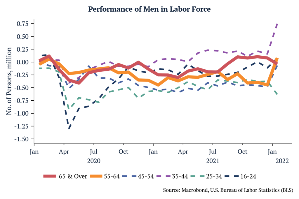
(3) Retirement is keeping people out of the labor force – It is hard to see that clearly in the data. The age group 55 and over (55-64 & 65 and over), suffered the least in both genders and have the least amount of people out of the labor force (when compared to January 2020 levels). Today there is 100k more men 65 and over in the labor force than at the peak in January 2020.