
Last week, just before the end of the month, we got the Second Quarter Advance GDP Estimate from the US Bureau of Economic Affairs (BEA). The quarter-over-quarter annualized number for real GDP printed a disappointing -0.9%, compared to a median expectation of +0.4%, but still better than the 1Q number of -1.6%.
GDP releases are very important events for markets. Companies use them to help make investment decisions, hiring plans, and forecast sales growth. Investment managers use them to refine their trading strategies. The White House and Federal Reserve both use GDP as a barometer for the effect of their policy choices.
These numbers are especially important for turning points in the economy. For some (but not the National Bureau of Economic Relations – the US agency responsible for classifying recessions), two consecutive quarters of negative real GDP growth is defined as a recession. If we took the early GDP releases at face value, this would imply that we are in a recession today, dating back to the first quarter. For all the above reasons, it is worth digging into how the BEA derives this number and how reliable the early releases are.
One of the tasks of the BEA is to calculate US GDP, measured as the total price tag in dollars of all goods and services made in the country for a given period. It is the sum value of all cars, new homes, lawnmowers, electric transformers, golf clubs, soybeans, barbeque grills, medical fees, computers, haircuts, hot dogs, and anything else sold in the US or exported during the period. When calculating current (or nominal-dollar) GDP, the agency adds the value of all goods and services in current dollars. But this herculean task does not end there, because what matters for most people is the real growth in the economy. And so, after tallying up everything in current dollars, the agency has to then make adjustments to try and come up with an estimate of the value of what was actually produced in the economy (e.g., ex-inflation).
Imagine an economy that only produces two things, potato chips and mobile phones. Suppose that the economy is selling $1.1 million of goods this year, an improvement of 10% compared to the $1 million from last year. That $1.1 million number represents the nominal GDP for the economy this year. But that number does not tell us how much of that 10% increase is due to more goods being sold and how much derives from price increases.
If last year there were 50,000 bags of chips sold for $10 and 500 mobile phones for $1,000, and this year there were 55,000 bags of chips and 550 mobile phones sold for the same price as last year, the economy had real growth of 10% and zero percent inflation.
Alternatively, if this year the economy sold the same number of chips and mobile phones as last year but did so at a price of $11 and $1,100, respectively, the economy had zero real growth and 10% inflation.
However, things are not so simple, for the methodology is designed not only to remove price inflation but also to adjust for the quality of the goods being sold. Let’s assume that this year the economy sold 55,000 bags of chips for $10, and 550 phones for $1,000 (the same as the first example). But in this example, the bags of chips sold this year only contain 40 chips versus the 50 chips in each sold last year, and the mobile phones sold this year have better computational power and an extra camera versus last year’s. In this case, the agency would have to account for those changes by calculating a positive price increase for the potato chips and a negative one for the mobile phones, even though the number consumers saw on the price tag did not change. Now imagine that the BEA must do this not just for all the goods sold in the US economy, but also for every service provided, and to deliver an advance estimate one month after the end of a quarter.
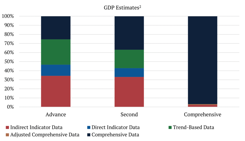
Which brings us to the question, how reliable are early GDP estimates? The answer is… it depends. Each revision incorporates more and better data and is believed to be a better estimate of the true value of GDP. For example, comprehensive data accounts for only 25.5% of advance estimates and 36.8% of second estimates, but it accounts for 96.7% of what we can call “final” estimates[1].
To assess the reliability of the GDP estimates we can look at revision patterns to understand if there is a bias in these revisions and how large they can be. To assess bias, we calculate Mean Revision (MR) where components tend to be offsetting and a large positive or negative number would indicate bias. To understand how large revisions can be, we calculate the Mean Absolute Revision (MAR) and the standard deviations, which are both complementary measures of the distribution for the revisions around their mean. We calculate these revision metrics for the Advance release that comes out one month after the end of a quarter, comparing with both, the Second releases (two months after the end of a quarter) and what we here call the “final” estimates (also called, comprehensive revisions, which are released approximately five years after the advance release).
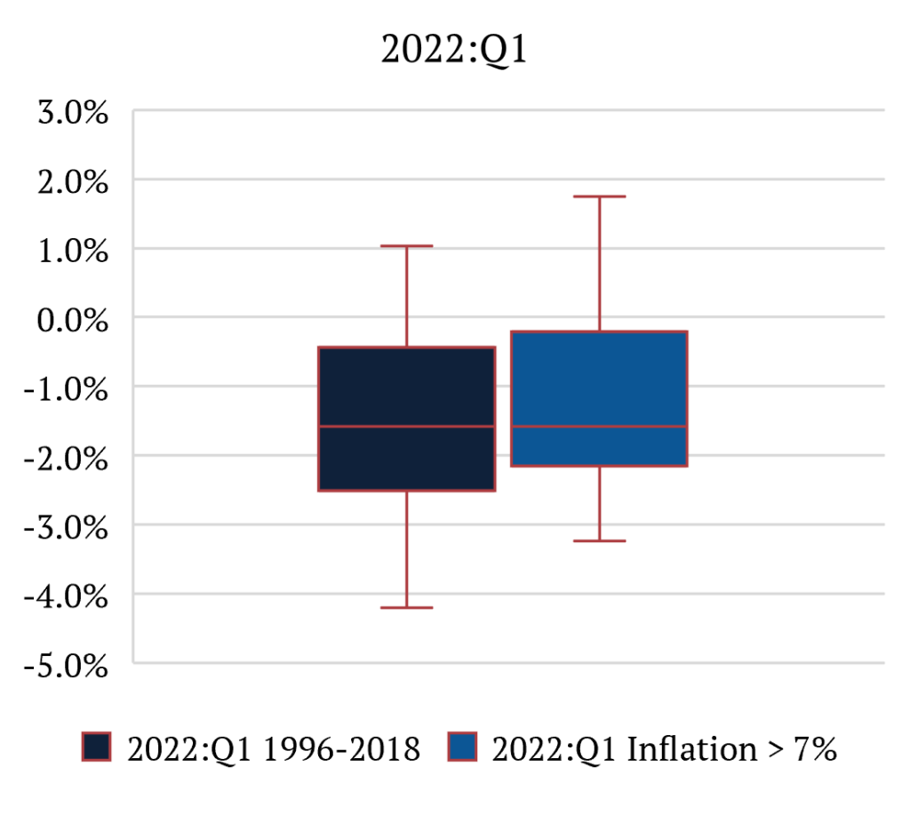
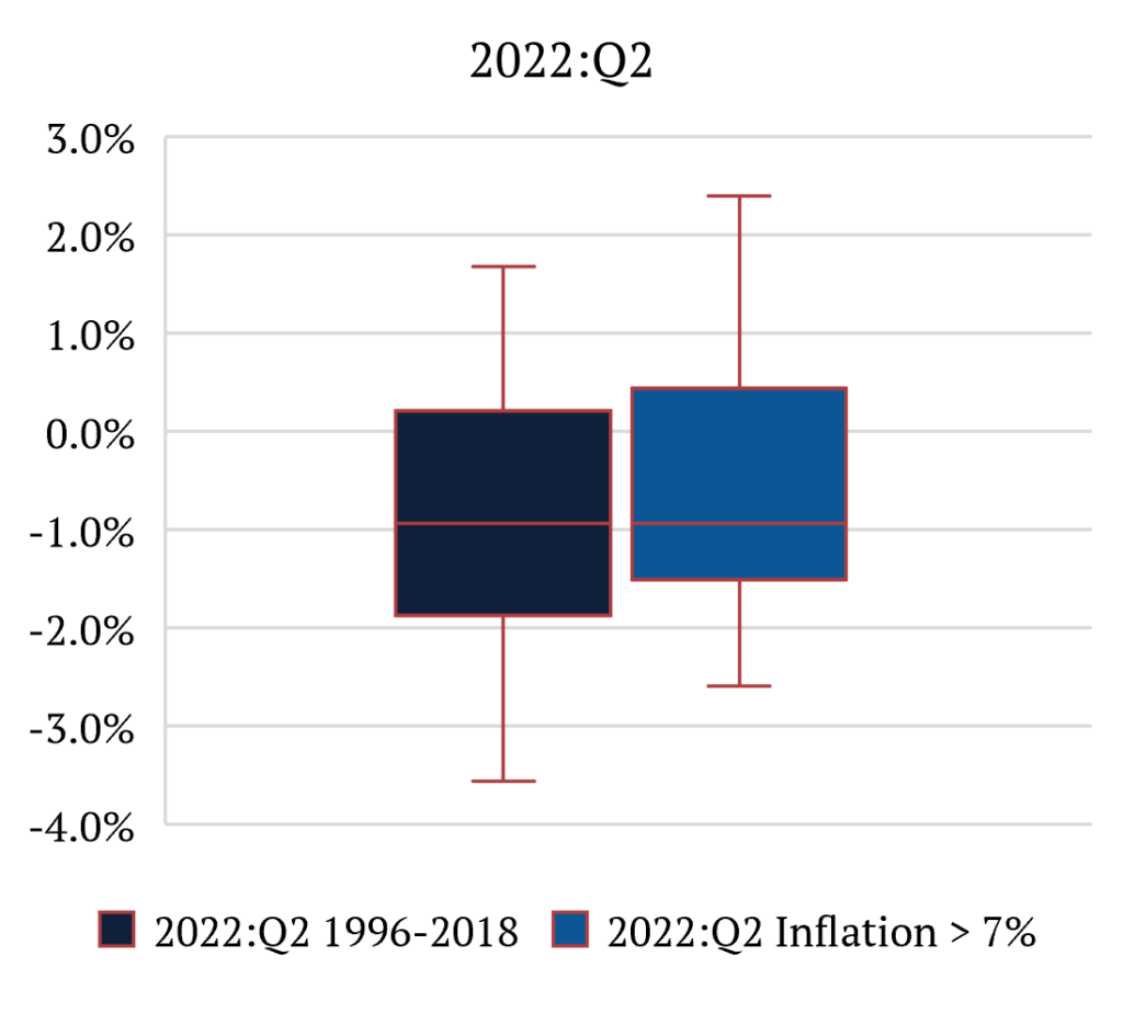
What we find is that inflation has a meaningful impact on reliability. More specifically, it creates a pronounced bias for advance releases in underestimating real GDP growth. This makes intuitive sense. The task of calculating real GDP becomes even more challenging during inflationary environments. Looking at the numbers, we find that in periods of low inflation [3,4], bias is virtually inexistent with MRs for Second and Final at +0.10% and -0.01%, respectively. While during periods when US CPI is above 7%, MRs are +0.40% and +0.80%, respectively. That means that, on average, in high-inflation environments, Advance GDP numbers are underestimated materially. It is also important to note that MARs and standard deviations are essentially unchanged from one environment to another. This means that the size of revisions is similar in both circumstances.
To clarify the point, let’s look at last week’s 2Q 2022 GDP Advance release of -0.9%. We can say that the second estimate will be between -1.5% and +0.4%, while the final estimate will be between -2.6% and 2.4%, with 90 percent confidence. This distinction between inflationary and non-inflationary environments is important because if we used the low-inflation scenario numbers, we would say that the second estimate would be between -1.9% and +0.2%, while the final estimate would be between -3.6% and +1.7%, with 90 percent confidence. [5]
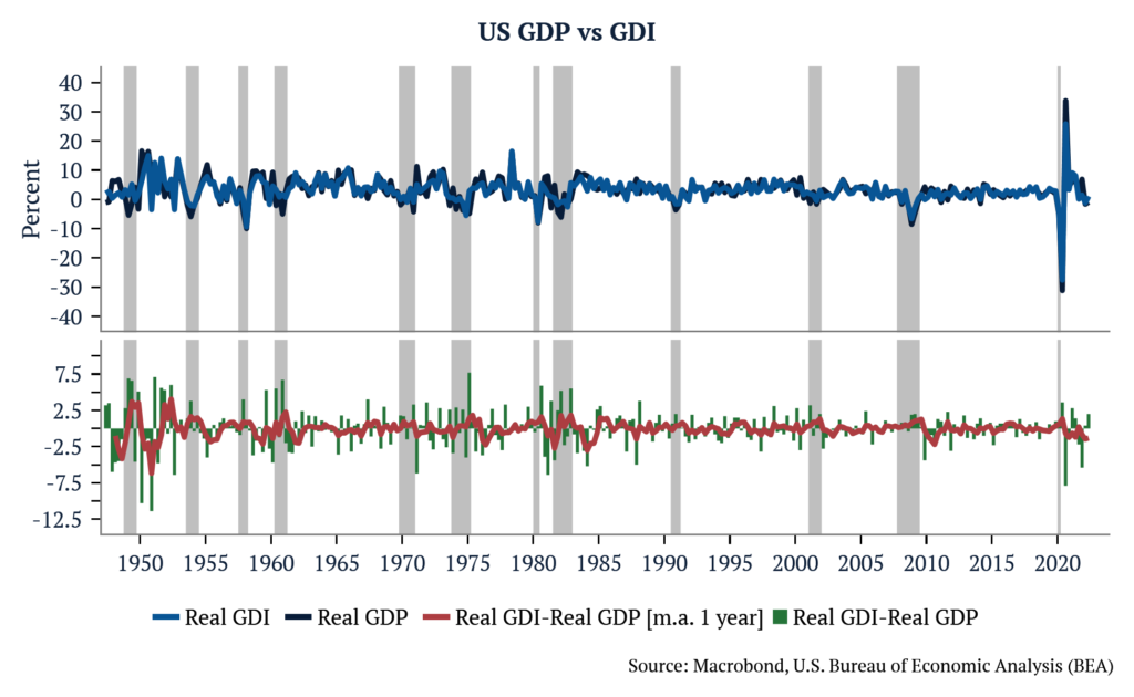
One way to increase the reliability of activity numbers is to look at the average of GDP and GDI. In theory, GDP and GDI should be equal, but in practice, GDP and GDI differ because they are constructed using different sources of information – both are imperfect in different ways. If both GDP and GDI are interpreted as the sums of unobserved, true economic activity and measurement errors, it is possible to infer that the weighted average series of the two is a more reliable measure of activity than either GDP or GDI alone, assuming some of the measurement errors are averaged out.
In short, calculating GDP is a mammoth undertaking, early estimates of real GDP tend to underestimate growth in inflationary environments, and you are better off taking a holistic view of the economy when data is as volatile as it is today.
P.S. We talked a lot about real GDP, but we should not neglect nominal GDP. Historically, S&P earnings growth tended to stay in line with nominal GDP. And that is how corporate sales, revenues, and profits are recorded. In the second quarter of 2022, nominal GDP in the US was approximately +7.9% QoQ annualized.
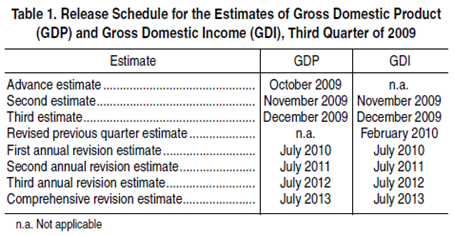
P.P.S. For a depiction of how and when GDP revisions and their vintages are made and maintained by the BEA, please see below.
[1] Comprehensive revisions are performed every five years and include major updates to classifications and definitions for the entire GDP time series – for more information, please see the endnote
[2] Holdren, Alyssa – Gross Domestic Product and Gross Domestic Income – Revisions and Source Data (June 2014)
[3] Fixler, Francisco, Kanal – The Revisions to Gross Domestic Product, Gross Domestic Income, and Their Major Components (June 2021)
[4] Using 1996-2018 period used in above paper, when US CPI inflation averaged 2.2%
[5] Revisions follow a normal distribution and therefore we can calculate the combined probability that the true value of real GDP growth in the 1Q and 2Q was below zero, i.e., two consecutive quarters of negative GDP growth. P (2Q < 0% | 1Q < 0%) = 36%.